


2 Impact of the factors of supply
When there is no scarcity of housing, the market is competitive and there is no reason for the existence of any price premium on a property.13 In a competitive market, all demand will be met with a supply. Around the world, there are cities with relatively high responsiveness of housing supply. In New Zealand, however, many studies estimate significant impacts from housing supply rigidities on housing supply and prices. For example, while the supply elasticity of New Zealand is estimated at 0.7114, the cities across the United States, with similar population density levels, have a supply responsiveness factor (supply elasticity) of 2.15
As presented in Figure 17, in response to increases in population, a rigid supply provides less housing (gross floor areas) and leads to higher house prices. As PwC (2020) discusses, the impact of supply rigidities is magnified during periods of faster population growth. PwC (2020) suggests that improving competitiveness in the land market such that the supplier of land and the consumers can compete across space and land uses, can lead to a less rigid housing supply.
Figure 17 Impact of rigid supply on house prices
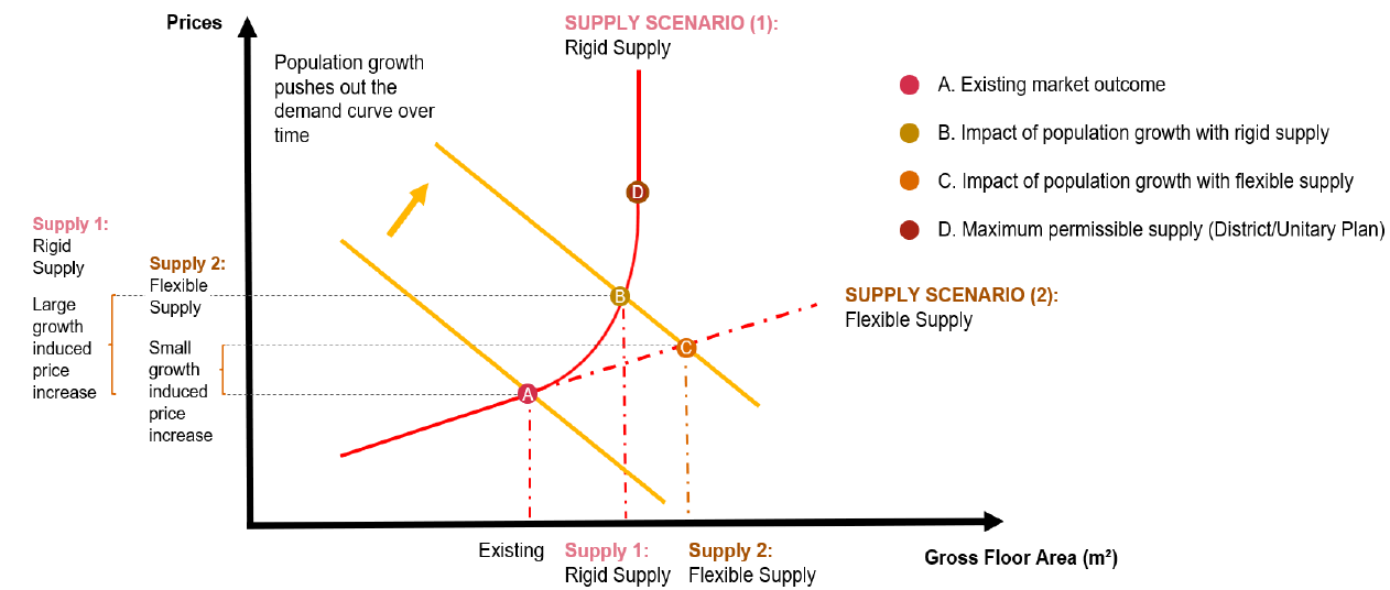
Source: PWC, 2020.
ANZ Research (2020) reflected on the supply issues; and discussed the existence of an infrastructure deficit and a significant housing shortage of between 60 and 120 thousand homes. They cited the scarcity of buildable land as an increasing problem, due to planning and zoning restrictions, land banking, urban-drift, poor infrastructure provision and other land-use pressures. We review the literature and discuss these factors further in the next sections.
There has been extensive literature on the impacts of factors of supply on house prices. Factors of supply have been discussed more thoroughly compared to the demand factors. There are multiple reasons that may have contributed to this:16
Most factors with direct impact on HPG are driven by the central and local government regulations. Most factors of demand have wider implications for the economy, with difficulties in measuring their impacts on HPG
Technically, capturing the impact of supply factors is relatively easier than capturing the impact of demand factors (given their wider implications for the economy)
There is a potential tendency for academic economists to replicate the work of their international peers, which is more focused on the factors of supply.
The lower responsiveness of housing supply (to a 1 percent increase in house prices) over time is an indication of the costly (restrictive) planning regulations
Grimes (2007) used a model (based on Tobin’s “q” approach17) to test the determinants of new housing supply. His results suggest that an increase in house prices by 1 percent (relative to total development costs) increases the new housing supply by a factor of between 0.5 and 1.1 percent.
We have listed the housing supply elasticity estimates available from the literature in Table 2. They capture the impact of a 1 percent increase in real house prices on the rate of new housing consented.18 Given this and the period of data coverage, the highest and lowest estimate of supply elasticities estimated in most of these studies provide information about the potential impact of planning policy within the RMA regulations.
The regional estimates using most recent data for Auckland, Hamilton, Tauranga, Christchurch and Queenstown suggest a decrease in the supply response to an increase in house prices over time.19 The reason for this decrease in supply elasticity can be geographic constraints, planning regulations, and technical constraints in the construction market (MRCagney et al., 2016; Saiz, 2010). We discuss this further in the next section.
Table 2 Housing supply elasticities
| Author | Auckland | Hamilton | Tauranga | Wellington | Christchurch | Queenstown |
|---|---|---|---|---|---|---|
| Sanchez and Johansson (2011) Nation-wide model (1994 -2007), Quarterly data | 0.705 | 0.705 | 0.705 | 0.705 | 0.705 | 0.705 |
| Grimes and Aitken (2010) TLA level (1991 -2004), Quarterly data | 1.000 | 2.900 | 1.200 | 0.200 | 1.100 | 3.600 |
| Grimes and Aitken (2006) National average (1981-2004) | 1.000 | 1.000 | 1.000 | 1.000 | 1.000 | 1.000 |
| (Hyslop et al., 2019) | 1.200 | 1.200 | 1.200 | 1.200 | 1.200 | 1.200 |
| PwC (2020) TLA level (1998 -2019), Monthly data | 0.876 | 0.840 | 0.517 | 1.353 | 0.778 | 0.875 |
Source: Sanchez and Johansson (2011); Grimes and Aitken (2010); Grimes and Aitken (2006); Hyslop et al., 2019; PwC, (2020).
2.0.0.1 The minimum cost of an irresponsive housing supply to the New Zealand economy is equal to 0.39 percent of its GDP ($1.3 billion per annum)
Nunns (2019) studied the socioeconomic impacts of rising house prices in New Zealand.20 His results suggest that a comprehensive removal of the housing supply constraint in New Zealand, with no trans-Tasman migration, will lead to an increase in per worker output by 0.8 percent (we review this study in more details in section 3.3). As the author mentioned, the study provides an indicative figure for the potential cost of a rigid housing supply. The lower land prices should be associated with allocation of capital (from other sectors of the economy) to lead to an increase in housing supply. This reallocation of the resources and the interaction between the housing sector (primarily the construction sector) and the other sectors of the economy needs to be investigated in a future study.21
To estimate the economic impact of the existing supply constraint, we used Nunns' (2019) estimate of the output per worker impact as an input to Principal Economics’ Computational General Equilibrium (CGE) Model. Our high-level estimate suggests that the annual cost of the supply rigidity in New Zealand is around 0.39 percent of its GDP.22 This is in absence of a potential increase in immigration to New Zealand as a result of a lower cost of housing.
2.1 Impact of regulations
Description
Regulation is the main tool of local and central governments affecting house prices.23 In theory, a more permissive regulatory regime increases competition amongst landowners, and is associated with a lower (or zero) speculation opportunities and lower house prices. Therefore, to reach a competitive land market has been the focus of the NPS-UD (2020).
In practice, the impact of regulatory barriers, institutional inefficiencies, and uncertainties associated with regulations are closely inter-related. Technically, the land price measure consists of elements of both costs and benefits of regulation. A higher price may be an indication of the benefits of councils’ services, such as improved access to amenities and facilities, or the costs imposed by inefficient regulations.
Summary of literature review
As we review in this section, several economic studies of the impact of regulation, provide estimates of the costs of regulation but there are relatively few studies that have examined the benefits of regulation. For example, there are many studies trying to estimate the costs of urban limit regulations, but there is no study identified of the potential benefits of urban limit regulation (through decreased negative externalities from urban growth on neighbouring regions). This is potentially because regulation is associated with difficult-to-quantify (social) benefits. Based on the literature, we know that a market-driven housing market, with minimal regulations, leads to lower house prices24 but it might have higher costs not expressed in the market.
From the available literature, it is not clear if the available resources in the economy, including capital, labour and technology required for construction of new houses, will be able to provide the size and magnitude of housing required for a flexible housing supply at a reasonable price.
Uncertainty assessment: restrictive regulation has led to higher house prices.

Lees (2019) assessed the cost of land use regulations using four different methods (inspired by Glaeser & Gyourko (2003). For this analysis he used detailed unit record house sales data sourced from Auckland Council and CoreLogic, with coverage for the 2012-2016 period. After accounting for a range of factors, including financing and council fees, his results suggest that house prices significantly exceed construction costs and that the price to cost ratios have increased over time. For example, between 2012 and 2016, the price to cost ratio in Auckland has increased from 2.72 to 3.37. During the same period, the ratio for apartments has increased from 2.62 in 2012 to 3.5 in 2016. His results for Christchurch and Queenstown are similar to Auckland. Lees (2019) concluded that the supply has not been responsive to prices.25 Using the same data and methodology, Lees (2019) estimated the cost of regulation in Auckland can be up to 56 percent of the cost of an average dwelling. Figure 18 shows his estimates of the cost of land use regulation.26 Lees (2019) discusses that the estimated cost of land use regulation could capture anything that drives a wedge between prices and construction costs, including the costs imposed by planning regulations and potential costs imposed from geographic restrictions, such as steep terrain in parts of Wellington and Queenstown. However, Lees (2019) argues that the likelihood of geographic restrictions being the driver of the price margin is low.27
Figure 18 Land regulation costs
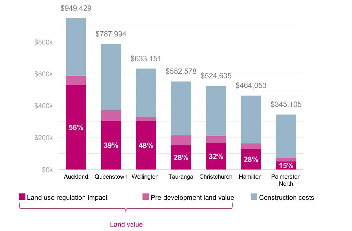
Source: Lees (2017).
A more competitive land market will increase competition between locations across a city and across different land uses. The decrease in the market power of landowners decreases land values. To achieve this, it is required that local governments promote development permission for both brownfield and greenfield developments, particularly in areas of high demand with better access to jobs. The results of a recent study by the Chief Economist Unit of Auckland Council confirm that more up-zoning (i.e. allowing greater housing density) is required to accommodate for the demand in areas closer to the city centre (Norman et al., 2021). The study does not account for the costs of supply in different locations.
In a comprehensive study of the costs and benefits of the NPS-UD, PwC (2020) estimated direct and indirect impacts of intensification, minimum car parking requirements, and local government’s strategic planning requirements. Their results suggest that the benefit to cost ratio (BCR) of achieving higher responsive housing supply (to price changes) across New Zealand cities is between four and seven.28
MRCagney et al. (2016) provides a comprehensive cost benefit analysis for policy options for the NPS-UDC. They investigated the impact of planning constraints including general zoning restrictions, MUL, building height limits, minimum parking requirements, apartment etc. Their results suggest that a less restrictive approach to urban planning that enabled sufficient supply to housing would reduce the rate of house price inflation by 50 percent with net benefits of $1.4 billion to $10.7 billion over the 2001-2013 period.
The viewshaft policy costs Auckland economy $1,366 billion
Cooper & Namit (2021) investigated the impact on house prices of Auckland’s viewshaft policies which restrict development to protect regionally significant views, to volcanos and the museum, for example. The CBD Viewshaft, for example, covers 1.7 million square metres of land. They used 2014 property (rating) data29 and viewshaft information from Auckland Council. The study uses a robust regression discontinuity method and accounts for the difficult to quantify benefits of viewshafts. Their results suggest that land values per square metre within 75 metres of the viewshaft are $1,282 higher than those located farther away (between 75 and 175 metres from the viewshaft boundary). Figure 19 shows the land values at different distances from viewshaft. Accordingly, for the properties located at the distance of 100 metre from the viewshaft, the estimated difference between land values per sqm for properties inside the viewshaft are on average $2,535 lower than the properties at the same distance located outside the viewshaft. After controlling for other features of land, the difference increases to $2,939. They conclude that the net cost from the viewshaft policy to the Auckland economy is $1,366 million (per year).
Figure 19 Land values and distance from viewshaft
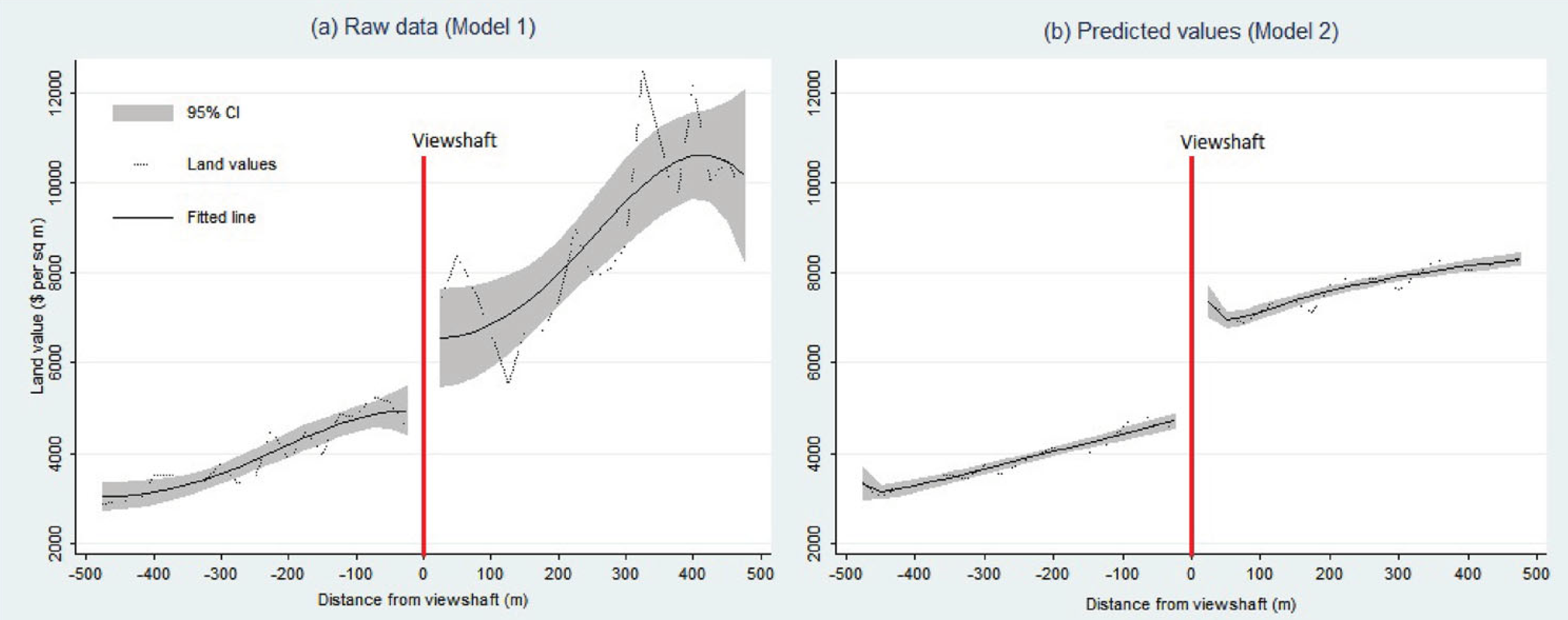
Source: Cooper & Namit (2021).
Grimes & Aitken (2006) studied determinants of new housing supply and the impact of supply responsiveness on price dynamics. Their results show that a 1 percent increase in house prices relative to total development costs raises new house supply with an elasticity of between 0.5 and 1.1 percent. Since the study has controlled for land prices, the estimated low response of the housing supply (to price increases) is likely driven by regulatory restrictions in the housing market. The authors also note that land prices have a strong impact on new house construction. A 1 percent increase in land prices is estimated to lift total development costs by 0.33 percent, which in turn leads to a 0.37 percent decrease in supply of houses. The data used is a quarterly dataset of median house prices for New Zealand over the period of 1991Q1 to 2004Q2 covering 73 Territorial Local Authorities from QVNZ. Given the lack of granularity of their data, the study does not provide more information about potential variations across location.
Greenaway-McGrevy (2018) assessed the impact of land use regulation on house prices in the Auckland region. They used a difference-in-difference (DiD) method and a unit level dataset of house sales for their assessment. The authors compared house price sales for property pre and post the Auckland Unitary Plan to test price effects of up-zoning (i.e., relaxing a restriction on site development). Their results suggest that up-zoning generated a significant increase in prices for underdeveloped properties relative to highly developed properties and properties that were not up-zoned; up-zoning in the most intensive residential zone generated a premium of 22.2 percent.
Parker (2015) uses the results of Bertaud, (2014) to show that Auckland’s population density is significantly higher in the CBD and almost flat in other areas. He discusses that the impacts of planning constraints are reflected by the non-continuous rate of population density in Auckland compared to other metropolitan areas (for illustration of the non-continuous density in Auckland see Figure 22). He argues that planning constraints that cause the need to build on progressively, more difficult sites lead to lower construction productivity. Additionally, planning constraints cause difficulties in buying large land areas for efficient scale development. Changes in population/dwelling density over time could provide more information about potential impact of policies. We will discuss this further in the next section, to provide an understanding of the potential impact of the RMA.
Grimes & Mitchell (2015) conducted interviews with 16 developers, providing information on 21 developments across Auckland to assess the costs of the rules and regulations (as perceived by developers).30 Their results suggest that building height limits and balcony requirements can each have costs impacts of over $30,000 per apartment. The council’s desired mix of typologies and increased minimum floor to ceiling heights can each add over $10,000 per apartment. For the residential section and standalone dwellings, infrastructure contributes not related to a specific development cost at around $15,000. These includes costs such as extended consent process, section size requirements, and other urban design considerations. They also assessed the potential loss in development capacity31 from council’s rules and regulations. Their results suggest a median loss in capacity of 22 percent (for the developments that proceeded).
Norman et al. (2021) used GIS mapping to illustrate that a higher land value correlates with high density housing areas. Assuming demand is highest at the city centre, they show that the Auckland Council’s zoning is not consistent with where demand is the highest.
Cavalleri, et al. (2019) use a stock-flow type model of supply and demand using panel data from 25-countries, between 1980Q1 and 2017Q4. They used an index as a proxy for land-use restrictiveness.32 Their findings suggest that: regulations that restrict housing tend to result in more vacant houses; regulations exacerbate mismatches between supply and demand; rent controls reduce the responsiveness of housing supply to demand pressures (though the effect is small); and that limits to urban expansion (geographic and regulatory) reduce incentives for new construction. > Mayer & Somerville, (2000) used quarterly data from a panel of 44 U.S. metropolitan areas between 1985 and 1996 to study the impact of house prices and costs on new housing construction. Their results suggest that metropolitan areas with more extensive regulations can have up to 45 percent fewer housing starts and price elasticities 20 percent lower than those in less-regulated markets. Also, their results suggest that a 1 percent increase in house prices temporarily increases new construction by 15 percent over current and following 5-quarters. The results of their modelling suggest that the regulations that lengthen the development process have an uneven temporal effect on supply elasticity.
Urban growth boundaries have led to HPG High agreement, High evidence
Based on the previous literature, the Productivity Commission's (2012) housing affordability inquiry, the price of land is responsible for between 40 and 60 percent of the cost of new dwellings in Auckland (in 2012) and is a driver of house price inflation. The inquiry refers to the results of a model that they estimated and identified the Auckland MUL as a driver of supply side rigidity. Our review of their model suggests that that there is a range of related factors that have not been accounted for in the model and may affect the results of their estimations. However, their results are consistent with the outputs of other studies using more comprehensive economic modelling frameworks.
Parker (2021) provides a comprehensive (theoretical) economic framework for the assessment of the impact of a competitive land market on house prices. His framework is based on a well-known economic modelling framework – AMM (Alonso-Muth-Mills model), which was widely used in previous studies in New Zealand.33 Parker discusses that, in an uncompetitive market, land prices on the fringe of the city depend on the bargaining power of households (demand for residential land) and farmers (demand for agricultural land). The output of his economic framework suggests that, in an uncompetitive land market, where there is a cap on the urban growth boundary, the price of residential land increases as a result of regulation, as illustrated in Figure 20.
Figure 20 Urban boundary limit leads to an increase in residential land prices
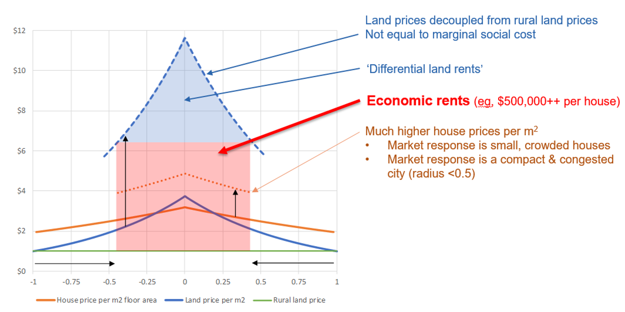
Source: Parker (2021). The horizontal axis shows distance from the city centre and the vertical axis is the price of land.
The prominent study of Grimes & Liang (2009) on the impact of the MUL on land prices has been cited widely as an indicator cost of regulation. We consider MUL regulation as an environmental regulation as its successor, the Rural Urban Boundary (RUB) under the Auckland Unitary Plan is denoted as a district plan land use rule pursuant to section 9(3) of the RMA. The authors study the difference in land prices between parcels located inside and outside of the urban boundary. Their results suggest that land inside the boundary is significantly more expensive than the land outside the boundary by a factor of between 7.9 and 13.2. As the authors noted, they do not have any information about the value of infrastructure that has been potentially capitalised into the land values inside the MUL.34 Also, the timeframe of the available data does not provide them any information about land prices before and after any MUL expansion. This study provides valuable information about the price increases associated with limitations imposed by MUL regulation.
Martin & Norman (2020) study the price difference between the land inside the RUB and the farm land outside the boundary.35 Consistent with the results of the previous studies, their study suggest the existence of a price premium for the land inside the urban boundary. However, their results suggest that converting farmland or lifestyle blocks into bulk-infrastructured residential sections would be unlikely to deliver land to the market substantially cheaper. Our review of the methodology of their study suggests that some of their assumptions have a significant impact on the results. For example, they refer to plans that suggest between 55 and 58 percent of land outside the urban boundary is unavailable for development, but they assume that only 35 percent of land outside the urban boundary is unavailable. This assumption is not justified and likely affects their results significantly. Our review of their methodology suggests that they have not used the location of the urban fringe in their analysis.
Zheng (2013) studied the impact of the MUL on land price. Consistent with earlier studies (for example, Grimes & Liang (2009)), his results suggest that the Auckland metropolitan urban limit results in upward pressure on residential land prices within the urban areas. His results show that the impact is uneven with a larger impact on land at the lower end of the price distribution. Also, when the supply of land on the urban periphery is restricted, the price of available residential land rises and new builds tend to be larger and more expensive houses.36
For the review of the impacts of the RMA and other regulations, it is important to differentiate between the impact of the regulation and the costs imposed from implementation of the regulations. The RMA categorises the activities that may exceed the limitations introduced by discrete plans to six categories, namely permitted, controlled, restricted discretionary, discretionary, non-complying and prohibited. The ‘activity category’ is a policy setting that determines the degree to which each element of a plan binds. The permission required for undertaking the activities that may affect the environment is called a ‘resource consent’ or ‘planning permission’. There is a chance of a regulatory impact on the probability of granting a resource consent. Torshizian (2015) defined ‘permissibility’ as the effective permission level granted by an activity status category. He investigated the permissibility of Auckland Council’s activity statuses and its impact on regional development. His results indicate that, once the characteristics of the activities are taken into account, a difference remains between the likelihood of different activity categories, and that interpreted as the bias associated with RMA regulation. Accordingly, the activity category ‘restricted discretionary’ (which restricts the scope of consideration to planners) is approximately 20 percent less permissive than ‘discretionary’, which is meant to be a more involved affair. His results suggest that the change in permissibility of the restricted discretionary activity has happened after the amalgamation in 2010.37 Also, after the amalgamation in 2010, the average likelihood of all activity statuses decreased by a factor of between -1.3 and -2.7 percent.38
Bassett et al. (2013) reviewed New Zealand’s housing affordability problem and the development of housing in New Zealand since the early 1900s. They provide a comprehensive review of the role of central and local governments in planning regulations over time. They argue that the lengthy and costly process of releasing land outside the Metropolitan Urban Limit (MUL) in Hobsonville, Flat Bush, Papakura, Karaka and Silverdale, between 1989 and 2010 was very costly (both in terms of expensive hearings and the social and economic costs of slow regional development).
Fernandez et al. (2020) studied the impact of proximity to Wetlands on residential property prices in Auckland. Their results suggest that proximity to natural wetlands is associated with lower house prices, but the interaction of artificial wetlands with parks is associated with higher house prices. They mention the importance of school zones on house prices, but do not account for that in their estimations. Their study does not account for proximity to other amenities and facilities and does not investigate causal relationships.
Cooper & Namit (2021) investigated the impact of Auckland’s viewshaft policies on house prices. Accordingly, the CBD Viewshaft covers 1.7 million square meters of land. Their results suggest that land values per square meter within 75 meters of the viewshaft are $1,282 higher than those located farther away (between 75 and 175 meters from the viewshaft boundary). They conclude that the net cost from the viewshaft policy to the Auckland economy is $1.4 billion (per year). The study uses a robust regression discontinuity method and accounts for the difficult to quantify benefits of viewshafts.
In an international study, Kallergis et al. (2018) investigates housing affordability across 200 cities.39 Their results suggest that a 10 percent increase in urban extent density leads to an 0.8 percent increase in price-to-income ratio. In the cities with enforced containment40 the price-to-income ratio is 1.6 percent higher than average. The advantage of this study is the large sample of the cities that they have included in their analysis. However, the analysis controls for a very few related variables to urban limit regulation and the results may not be interpreted as causal effects.
Table 3 Difference in land values across the RUB
| Author | Multiplier | Notes |
|---|---|---|
| Grimes & Liang (2009) | 7.9 – 13.2 | Controlling for area unit effects found a boundary effect of 5 – 6 in 2001. However, is likely to reduce the estimated boundary impact and underestimate results. |
| MBIE & MfE (2017) | 3.15 | Auckland is 3.15. Ratios of 1.53 - 3.15 depending on geographic area. |
| Zheng (2013) | 1.3 - 9.7 | Lowest price decile 9.7, Median price 5 Highest price decile 1.3 |
| Productivity Commission (2012) | 7.15 - 8.65 | 7.15 in 1995, 8.65 in 2010 |
| Martin & Norman (2020) | 0.006 – 0.052 | For residential-sized lands inside the Auckland RUB 2020. |
Source: Grimes & Liang (2009); MBIE & MfE (2017); Zheng (2013); Productivity Commission (2012); Martin & Norman (2020).
The studies reviewed above have discussed the impact of regulation on house prices. The literature on the impact of regulation on house price growth is limited. Torshizian (2018) estimated the impact of MUL expansion on house price growth in the Auckland region. This is the only study that captures the impact on prices of houses located in different proximities to the expanded area, before and after the expansion. The study captures the impact for the suburbs located nearby the expanded area and compares that with the suburbs with similar opportunity to expand. For benchmarking, the study uses the price growth of houses compared to the houses with similar price range located in the central area (which are not directly affected by an urban expansion). Results suggest that:
the price growth in expanded areas is similar to the central areas,
the price growth in areas nearby the expanded area is similar to the other areas with similar features, and
the price growth outside the urban boundary is significantly higher for areas located closer to the expanded area.
The author concludes that the reason for high price growth in the areas located outside the boundary and nearby the expanded area, is their expectation of future growth in their area.41
This expands the findings of the other studies by providing evidence for the lack of competition in the land market being a driver of house price growth. Accordingly, the lack of competition resulting from the MUL is associated with an average of 13 percent higher house price growth. This is equal to an average of 0.31 percent additional cost to the land values, which is equal to $4,730 (in 2021-dollar values).
Geographic constraints have not been the driver of HPG High agreement, Medium evidence, Medium certainty
As described, many studies of the regulation impacts do not directly account for the impact of geographic constraints. This is due to measurement issues. Given the robust economic assessment framework that these studies used and the high agreement across the studies, we conclude that the impact of geographic constraints on the findings of the studies of costs of regulation is insignificant.
Saiz (2010) investigated the impact of geographic constraints on urban development using GIS derived data (coastal areas and land steepness) for metropolitan centres in the U.S. over the period of 1970 – 2000. The findings show geographically constrained areas tended to be more expensive, with faster price growth. Furthermore, antigrowth local land policies are more likely occur in growing land-constrained areas.
Nunns (2019) provides an estimate of the likely costs imposed by geographic constraints. He defined geographic constraints as a lack of flat developable land.42 His results suggest that a 1 percent increase in geographic restrictions is associated with $39 per sqm higher land prices.
2.2 Impact of the RMA and environmental regulations
Description
The RMA and environmental regulations impact housing through their guidelines for councils’ planning regulation developed based on the RMA. Currently, the RMA is going through a reform. A successful reform will support the NPS-UD agenda, by improving the competitiveness of urban land markets43, and go beyond the requirements of the NPS-UD by providing a more certain regulatory framework that will lead to higher certainty around planning regulations.44
Summary of literature review
The literature on the impact of environmental regulation on HPG is limited. This is partly because of the overlapping impact of the RMA and the planning regulations. For example, it is not clear how much of the costs imposed from an urban-rural boundary regulation are because of the environmental limits imposed by the RMA versus the planning targets of intensification. The limited literature on the impact of environmental regulation is not supported with strong evidence. However, there is high agreement in the literature that a more transparent, permissive and well-monitored resource management regulatory regime leads to lower social costs through its impact on the planning regulations.
Most of the literature we include in this section is based on conference and policy papers and a parallel study of the impact of Resource Management reforms. For a robust understanding of the impact of RMA, we need further robust assessments using granular geographic data. The interaction between the environmental regulation and other legislations (and infrastructure planning) needs further investigation.
Uncertainty assessment: RMA has led to HPG (or the driver of costly planning regulation is RMA

There is not a clear distinction between the impact of environmental and non-environmental regulations. The impact of environmental regulation is mainly on the land use, which is expressed as the reason for the zoning regulations. The primary impact of land use regulation is on urban growth boundaries (at the periphery of the city) and the resource consents’ level of permission for different activities. The linkage between the zoning regulations and the RMA, however, is not supported with evidence. We reviewed the literature on the impact of urban growth boundaries in the previous section. While the urban growth boundary is not a restriction (directly) imposed by the RMA, a successful resource management legislation must provide clear instructions about its implications for the planning regulation (and monitor correct implementation).
Parallel to this review, Resource Economics, Principal Economics and Sapere (2021) assess the impact of RM reform. They discuss that the outcomes of councils’ planning regulation (driven by the NPS-UD), if accompanied by a permissive and transparent RM system, can lead to higher benefits than those from the NPS-UD alone. As shown in Figure 21, the combination of the features of the RM system and their interactions with the councils’ regulation may lead to a wide range of outcomes for the housing market.
Figure 21 Combined impact of RM system and planning regime

Source: Principal Economics.
The pattern of dwelling density in Auckland before and after the RMA effects come to existence in 1991 are shown on the left-hand side of Figure 22. As illustrated, the pattern has changed dramatically over time.45 This is consistent with the changes in pattern of land values illustrated on the right-hand side of Figure 22. The comparisons between the two graphs shows the high correlation between patterns of dwelling density and land prices over time.46
As shown in Figure 12, there has been many legislative changes over the 1980-2020 period that may have been associated with this change in the distribution of houses and prices. For example, the RMA and the local government reforms in 1989 led to widespread changes across New Zealand local governments. The 1989 reforms led to a decrease in the number of local governments by 90 percent (from 828 to 86 in 1989). The RMA played a complementary role to the 1989 local government reforms. There is a more careful assessment of the impact of the two reforms on providing enabling and effective development outcomes required.

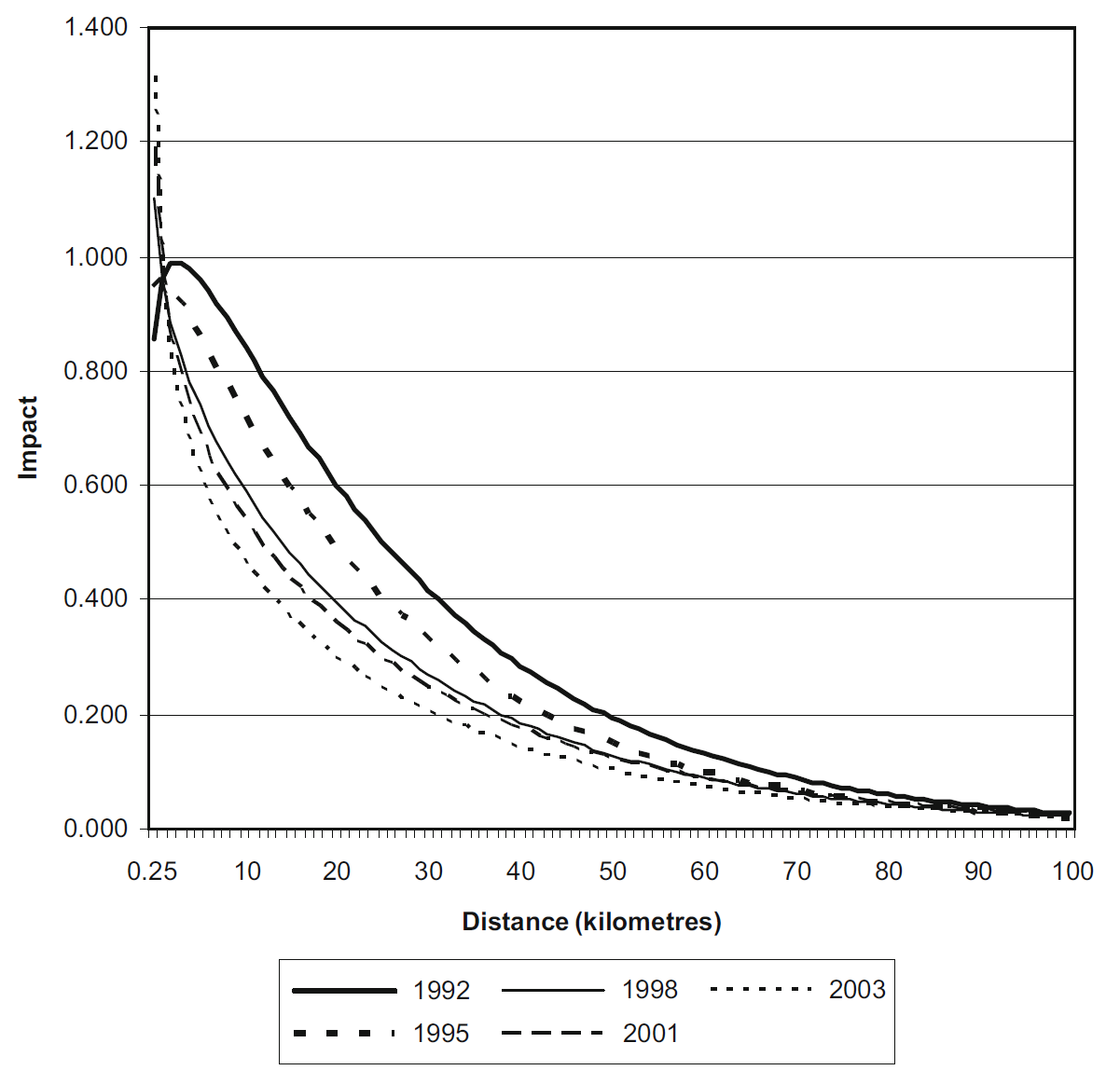
Table 4 High level housing outcomes of NPS-UD and RMA and the RM reform
| Outcomes | NPS-UD & RMA | RM reform |
|---|---|---|
| Affordability | NPS-UD has a range of recommendations contributing to housing supply elasticity, including:
competitive land markets and high-quality greenfield development |
- National direction and more clear legislation leads to decreases in consenting cost which translates into allocative efficiencies - Housing supply is responsive to demand, with competitive land markets enabling more efficient land use and responsive development, which helps improve housing supply |
| Choice | Improving housing choice through: - increasing planning flexibility. - aiming for agglomeration benefits – i.e. larger or denser places tend to provide greater variety of services and consumer goods |
Increase housing supply to better meet residents’ demand for housing (by type, size, location and price) |
| Māori participation | Recognise Te Tiriti and contains provisions aiming to enable Māori participation in the system | - Enabling the housing aspirations of Māori such as by enabling papakāinga developments - Providing opportunity for Māori to participate as Treaty partners across the RM system, including in national and regional strategic decisions. Māori will be sufficiently resourced for duties or functions that are in the public interest |
| Climate change | Better prepare for adapting to climate change and risks from natural hazards, and better mitigate emissions contributing to climate change | A reduction in transport carbon emissions versus the status quo from more efficient land use patterns through improved spatial planning |
| Improved System performance | Focused on improving effectiveness of planning regulations | Improve system efficiency and effectiveness, and reduce complexity, while retaining appropriate local democratic input |
The RMA reduces the responsiveness of housing supply high agreement, medium evidence, medium certainty
A successful RM system provides:
a regulatory framework that leads to higher certainty around zoning regulations.
a more flexible housing supply through providing a more permissive regulation and allowing more flexibility in housing supply.
Given the complementary roles of the RM system and the NPS-UD, Resource Economics et al (2021) discuss that the total impact of the RM system and NPS-UD is to achieve a responsive housing supply. To distinguish between the impact of the RM system (and the reforms) and that of the NPS-UD, we can use estimates of the impacts of an improvement in the resource consent process and its impact on land values. Any impact on land values in addition to the estimated impacts of resource consent is likely driven by the NPS-UD.
The RM system (and the reform) provide a national level direction (or centralisation). This leads to a decrease in the chance of negative externalities from one region’s urban growth on other regions;47 and an increase in certainties around permitted and prohibited activities (with less room for discretion). Also, one of the objectives the reforms is to decrease the number of Acts to resolve any potential inconsistencies across different pieces of legislation leading to a higher certainty/transparency level.
Torshizian (2015) estimated the likelihood of granting a consent to different activity statuses after accounting for the features of the applications. He argues that the likelihood of granting a consent should be similar across all activity statuses after accounting for the features of the application. After accounting for the likelihood of not applying for a consent due to its high processing cost (as a combination of time required for processing a consent and the associated fees), his results suggested that the activity category ‘restricted discretionary’ (which restricts the scope of consideration to planners) is approximately 20 percent less permissive than ‘discretionary’, which is meant to be a more involved affair. This figure provides an estimate of the impact of improved certainty on the likelihood of granting a consent.48
The results of that study suggest that a 1 percent increase in the processing delays is associated with 1.4 percent lower likelihood of granting a consent. To capture the affordability impacts of lower consenting likelihood, we use the results of Nunns (2021), which suggests that a 1 percent higher likelihood of consent processing delays is associated with $24 per sqm increased costs (in term of land price distortions). Using these multipliers suggest that a 1 percent lower likelihood of granting a consent is associated with $17.1 per sqm higher prices. Figure 23 shows the relationship between the number of processing days of a resource consent application and the likelihood of granting a consent. Accordingly, the chance of granting a consent decreases significantly as the processing time increases.
Figure 23 Impact of processing delays on the likelihood of granting a resource consent
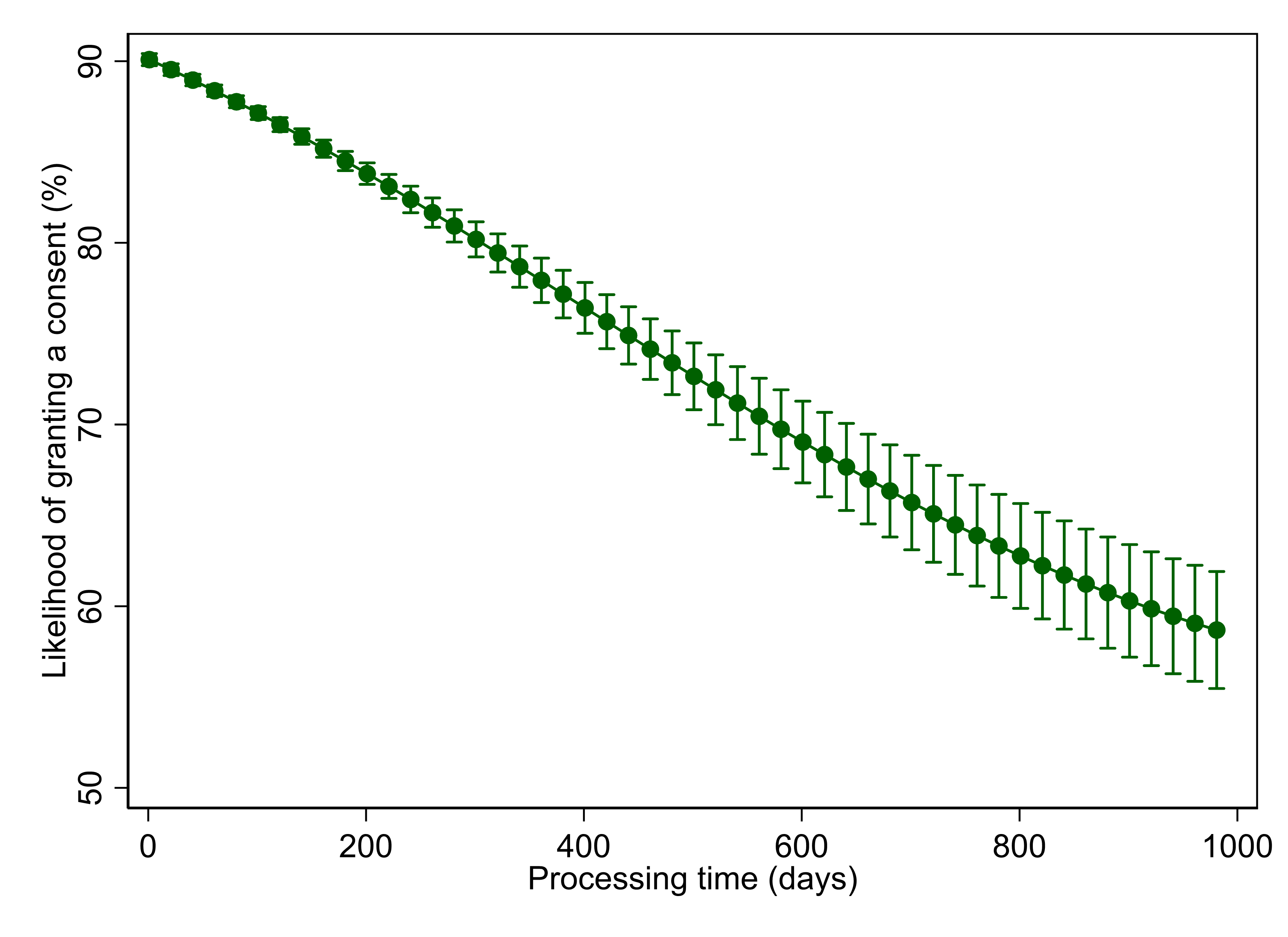

Source: Auckland Council; Torshizian (2015) on the left hand side show the relationship between 2005 and 2015; Principal Economics analysis on the right hand side shows the relationship for the 2005-2021 period.
Resource Economics et al. (2021) discuss that centralisation (potentially resulted from increases in national direction) depends on its contribution to the objectives of the NPS-UD. A successful centralisation leads to efficiency gains and significant economic and social benefits. However, an inefficient centralisation will be associated with negative outcomes.
Torshizian (2015) investigated the likelihood of granting a consent for different activity statuses before and after the amalgamation in Auckland. His results show that after the amalgamation in 2010, the average likelihood of all activity statuses decreased by a factor of between -1.3 and -2.7 percent. This figure captures the potential negative impact on urban development from a lower opportunity to compete for attracting urban development opportunities to the region. While this figure provides an indication of the impact of centralisation in local government, it provides an overall estimate of the likely inefficiencies involved in centralisation.
There are potential gains from improved certainty resulted from national direction. As discussed, the NPF’s greater (mandatory) national direction leads to improved prioritisation of national outcomes and better governance of potential negative externalities. Improved prioritisation means that the planning regulation will redirect investments to the projects with the highest expected return on investment, after accounting for financial, economic and social outcomes. This means that the combination of the RM system and its impact on planning regulations will lead to a responsive housing supply.
A more responsive housing supply is driven by competitive land market, which is mainly affected by the urban growth boundary regulation and the (other) planning regulations. It is not clear to what extent these regulations are affected by the RMA. However, an effective RM system clarifies the need for efficient planning regulation, which will lead to a competitive land market across New Zealand. The reform requires Councils to provide infrastructure in the areas of future growth. The reform also clearly identifies the environmental limits. Given the environmental constraints and the high demand, the councils will need to relax a wide range of costly regulations to accommodate for the future growth. This includes two broad set of policies on the urban growth boundaries and the other wide range of zoning regulations.
The likely changes in land values resulted from a successful RM system (through the RM reforms) in Auckland are shown in Table 5. These parameters change slightly across regions, depending on the average land values. As illustrated, a 100 percent increase in transparency is associated with 4.17 percent lower land values through its impact on resource consents. Centralisation (or national direction) is associated with 0.41 percent higher land values, in the absence of its potential positive impact on competitive land markets (CLM). The impact of CLM through less stringent Urban Growth Boundaries (UGB) is a decrease in average land values by 0.23 percent. The rest of the impact of removal of the housing supply constraint is captured through the other regulations. This impact may still be affected by the RMA, through a more prescriptive regulatory regime and improved alignment with infrastructure planning.
Table 5 Likely impact of the features of RM system on land values
| Objective | Impact on land values (%) | Source | Impact of RMA |
|---|---|---|---|
| Transparency | -4.17 | Torshizian, 2015 ; Nunns, 2021 | Yes |
| Centralisation | |||
| - In isolation | 0.41 | Torshizian, 2015; Nunns, 2021 | Yes |
| - CLM - UGB | -0.23 | Torshizian, 2015 | Yes |
| - CLM - Other | -17.60 | Principal Economics analysis using results of Grimes & Mitchell, 2015 | No |
| Total | -22.00 |
Source: Torshizian (2015); Nunns (2021); NZIER (2014); Grimes (2015); Principal Economics analysis.
MRCagney et al. (2016) referred to the complementary role of planning regulations and infrastructure planning, funding and provision. They emphasised on the importance of improved coordination between planning regulation and infrastructure planning, which are governed by separate legislation, to provide the infrastructure in the right place and at the right time. This has been recognised as an objective of the RM reform.
In addition to their discussion of the impact of urban growth boundaries and other regulations that we reviewed in the previous sections, also discussed development levies. They noted that the RMA sets strict rules about the relationship between development levies collected and how they were spent, but councils have sought the widest interpretation of the rules. They do not provide data but refer to some examples in Auckland. A successful RM reform will provide transparency and minimises the chance of any misinterpretation.
2.3 Availability of infrastructure
Description
Having the infrastructure capacity required for providing more housing is a driver of house prices. One reason for less permissive regulations is the lack of infrastructure to support the brownfield and greenfield growth. Hence, the correct timing of the provisions of infrastructure contributes to an increase in housing supply and leads to a lower house price (growth). There are multiple issues with the provisions of infrastructure, particularly around the inefficient decision making around infrastructure investments.
Summary of literature review
As discussed extensively in the literature, the lack of infrastructure is a significant barrier to housing supply. The funding and financing issues and the potential inefficiency of the local government have been cited as the drivers of infrastructure shortage. There have been discussions of the importance of further alignment between legislations, particularly between the RM system and infrastructure planning, to ensure efficient outcomes from infrastructure investments. The empirical evidence on the efficient use of the available infrastructure and its interaction with other factors of supply, particularly planning regulations, is limited.
Uncertainty assessment: Lack of infrastructure has led to HPG.

New developments require large upfront investments by councils or developers. Infrastructure can be a bottleneck (McEwan, 2018; Productivity Commission, 2017).49 Mechanisms to connect benefits and costs of growth struggle to provide sufficient infrastructure even if the land is suitable for house building (Johnson et al., 2018).
The long-lasting impact of infrastructure and the importance of planning ahead
The NPS-UD requires local councils to provide sufficient feasible development capacity in resource management plans and support that with infrastructure.50 The NPS-UD uses the Future Development Strategy (FDS) process for ensuring that the planning processes provide enough development capacity to meet future growth needs. The objectives of the FDS are to:
improve the alignment between spatial planning and land-use and infrastructure planning51
inform RMA plans and other relevant legislation
promote a well-functioning urban environment, informed by the values of iwi and hapū
The FDS tasks councils to provide information about the location of future development and timing of infrastructure investment. The objective of the FDS is to minimise infrastructure costs and prevent severe rises in house prices. To achieve this, the NPS-UD recommends developments in areas with high accessibility to jobs, urban amenities and transport technologies. This is consistent with the housing specific objectives of the RM reforms to provide the right infrastructure, in the right place at the right time, that provides adequate access to economic and social opportunities and enables people to maximise their wellbeing.
The lack of infrastructure has been noted as a constraint that has led to zoning restrictions (Grimes & Liang, 2009; Martin & Norman, 2020). Bassett et al. (2013) provided an estimate of the council costs for roads, footpaths, drains, and other infrastructure at around $85,000 per section, the cost of water and sewerage at around $20,000 per house and the cost of building consent at around $40,000 per house. Except for the cost of building consent, which is sourced from the Statistics New Zealand Official Yearbook (2008), the authors do not provide their calculations/sources for other cost estimates.
Bassett et al. (2013) discuss the monopoly power of local councils in both granting consents and providing infrastructure. They questioned the efficiency of this system in terms of providing infrastructure required for growth and being accountable for that. They specifically refer to the monopoly power of Watercare in Auckland and its power in extracting rents out of developers and not being accountable to ratepayers.
Skidmore (2014) compared New Zealand housing trends and policies with those of the United States. The author cited Albouy (2009) on how the US urban area price differential between undeveloped and developed land on the fringe is about equal to cost of converting agricultural land into development (i.e. costs of infrastructure). The author notes that development contributions offer a needed source of infrastructure funding but may also increase housing prices and reduce the construction of more affordable and dense development.
The costs of infrastructure have been noted as a prohibitive factor for recent developments. Grimes & Mitchell (2015) documented the costs of the rules and regulations as perceived by developers. Auckland developers responding to a survey noted that they were asked to fund key community infrastructure beyond that directly related to their own project. Additionally, developers feel that Watercare and Auckland Transport were engaging in monopolistic behaviour to force them to fund upgrades and expansion of infrastructure where the benefits extended beyond their development. Some developers abandoned their projects due to issues over access to infrastructure or cost of upgrading the existing infrastructure. Availability of infrastructure caused 13 percent of respondents to abandon a project and 38 percent noted the costs of providing infrastructure influenced abandonment.52
The Productivity Commission’s (2012) housing affordability inquiry suggests that the monopoly power of councils in providing infrastructure to service land and the access to development contributions may incentivise councils to designs that have higher initial capital expenditure.
The Productivity Commission (2017) inquiry into better urban planning suggests that supply is rationed reflecting perceived difficulties in financing, recovering costs and burdening existing residents. Limited supply is often the binding constraint to meeting demand for development in high-growth cities. The inquiry calls for more cohesive plans linked to infrastructure supply, market-based tools and infrastructure pricing. The inquiry recommends that the long-term infrastructure (and land-use planning) needs to account for the uncertainties involved in the decision-making process. MRCagney et al. (2016) cited BERL (2016) for the RMA planning process (and infrastructure provision) contributing to a very long time for converting land from current zoning to new business use. Some participants suggested 7 to 15 years to complete this process.53 Parker (2015) noted that houses cannot be built without costly infrastructure that takes time to plan and deliver with funding and financing challenges. In a study parallel to this review, Principal Economics (2021) is estimating the costs imposed on the economy from inefficiencies in the decision-making process.
As noted by the Productivity Commission (2017), councils have faced difficulties recovering the full costs of infrastructure from those creating the demand. This has led many councils to ration the supply of new infrastructure, contributing to scarcity and higher land and housing prices. Further investigation of the politically and practically sound funding and financing solutions is currently underway.
Figure 24 shows the changes in (real) Producers’ Price Index Outputs for the 1995-2021 period.54 Accordingly, the operating costs of the infrastructure sector has increased gradually over the last two decades (between 2000 and 2020) by 22 percent.
Figure 24 Real PPI – Heavy and civil engineering construction

Source: Bank for International Settlements, Statistics NZ, Principal Economics 2021 analysis.
Note: We source s.a. real property price index from The Bank of International Settlements, PPI for heavy and civil engineering construction from Statistics NZ and adjust for inflation using the CPI from Statistics NZ. We then calculate the year-on-year annual change for each series. We highlight notable recessionary periods in New Zealand identified by Reddell et al., (2008). These include the First Oil Price Shock (1974 – 1977), The Second Oil Price Shock (1979 – 1982), The 91 – 92 Recession (attributable to the 1987 share market crash, subsequent monetary responses and impacts of the first Gulf War - 1991 – 1992), The Asian Crisis and drought (1997 – 1999), we add COVID-19 as an additional recessionary period (2020-).
2.4 Supply chains and construction costs
Description
Increases in construction costs are driven by the higher cost of materials (following a change in building codes, for example), increased cost of labour (due to skill shortage or low labour productivity), lack of suitable technology (such as modular housing technology), the small scale of the construction sector (which is a function of regulations, size of demand and all other factors).
Summary of literature review
The literature on the impact of construction costs and supply chain provides information about the accounting costs of constructing a new house. The literature, however, does not provide a robust conversation about the interactions between construction costs and all other related factors, such as changes in technology, the impact of planning regulations and the scale of the construction sector.
Uncertainty assessment: The increased construction cost and the supply chain issues have led to HPG.

Based on the Productivity Commission (2012)’s housing affordability inquiry, between 2002 and 2009 the changes in material costs for a standard home have increased 20 percent in real terms. Half of that increase in costs was due to the introduction of new materials. Increasing building code requirements have led to an increase in construction costs which has a direct impact on housing prices. This is consistent with other studies, such as Bassett et al. (2013), which suggest that the changes in the building codes have led to an increase in costs and have been associated with increased quality of the housing.
Johnson et al. (2018) discussed that the poor performance of the construction industry and land development sectors can partly be attributed to misguided or indifferent public policy. Accordingly, the average construction cost of an ‘average house’ has risen by 28 percent over the 2012-2017 period and by 180 percent over the period of 1997-2017.55 They argued that the development and construction sectors are small scale, low productive and prone to boom-bust cycles, and upheavals in funding and land banking. Cyclical uncertainty discourages investment technologies like pre-fabrication, long-term planning and training of apprentices. They also argued that labour shortage is a significant problem for the construction sector as during busts many firms fail and workers migrate to Australia or leave the construction sector entirely. Their arguments are based on their expert advice.
Denne et al. (2016) discussed the factors of a competitive housing market to support the NPS-UDC. Accordingly, the high costs of building reflect a number of barriers and lack of competition in some construction markets. They discuss that in a competitive market, price-taking developers seek to maximise their profits by minimising development costs. This means building up until marginal construction costs are equal to average costs. Consequently, the study suggests that large, persistent deviations from marginal construction costs indicate that building height limits are constraining development and distorting prices.
In addition to his discussion of the cost of regulation, Parker (2015) reviewed the useful housing policy instruments and suggested that the cost of building has increased. He named a few reasons for the higher construction costs, including the need to build in progressively more difficult sites, liability rules for the industry, heavily involvement by councils and possible market issues. Grimes (2007) modelled the determinants of new housing supply. Accordingly, a 1 percent increase in land prices is associated with an increase of 0.33 percent in total development costs, which leads to 0.37 percent decrease in housing supply.
Samarasinghe (2014) studied the nature of the material supply chain in the New Zealand residential construction sector. He conducted 30 interviews across the supply chain in the Auckland region. His results suggest that the construction industry uses traditional procurement strategies and that the material supply chain management process is sub-optimal. His results show that the price of building material in New Zealand is high, products are inferior, houses are very customised, transport costs are high, and labour costs are high. He suggests increasing the standardisation of residential building as a solution. He also suggests a web-based building materials information system can improve collaboration in the supply chain. The results of this study are based on the interviews conducted and provide limited robust evidence for improvement of the supply chain.
Skidmore (2014) compared New Zealand housing trends and policies with those of the US. The author notes that the construction firms in New Zealand tend to be small because of land use regulations which constrict the ability for large scale land acquisition. The approval process for large scale development makes approval length and variable and uncertain, with significant delays due to various factors including local government approvals can lead to significant financial stress and even bankruptcy. This uncertainty and scale of upfront costs can make it difficult for construction companies to grow. This study is not evidence-based.
As discussed by Brebner (2014), the building Act of 1991 may have slowed construction and added costs to homeowners. The small size of construction firms, lack of innovation and desire for bespoke homes in New Zealand has not helped house prices. The author also discusses that the size of the building industry in New Zealand is small, with 45 percent of the builders being self-employed in 2010. They suggest that innovative construction methods, such as building modular units, as a good solution for improving the efficiency of the building sector.
Grimes & Aitken (2004) studied the impact of a range of factors on house prices using a macroeconomic model. Accordingly, the real construction costs have an asymmetric effect, being significant in buoyant times but not in depressed times. This may suggest that with the improved regulatory framework, and a more elastic land supply, there will be limits on the availability of inputs for the constructions sector to supply more housing.
Figure 25 shows the growth in the construction costs over the 1995Q2-2020Q4 period. During this period the cost of construction grew by 39 percent, and the housing prices increased by 124 percent.
Figure 25 Construction costs % change, PPI – Residential building construction

Source: Statistics New Zealand, Bank for International Settlements, Principal Economics 2021 analysis.
Note: We source s.a. real property price index from The Bank of International Settlements, PPI for residential building construction from Statistics NZ and adjust for inflation using the CPI from Statistics NZ. We then calculate the year-on-year annual change for each series. We highlight notable recessionary periods in New Zealand identified by (Reddell et al., 2008). These include the First Oil Price Shock (1974 – 1977), The Second Oil Price Shock (1979 – 1982), The 91 – 92 Recession, (attributable to the 1987 share market crash, subsequent monetary responses and impacts of the first Gulf War - 1991 – 1992), The Asian Crisis and drought (1997 – 1999), we add COVID-19 as an additional recessionary period (2020-).
This is based on an assumption of housing being a homogenous good. In practice, the features of land and housing are often unique to each parcel/house and that leads to a price premium for the scarce features↩︎
i.e. with 1 percent increase in house prices, the housing supply increases by 0.71 percent↩︎
This is based on Sánchez & Johansson’s (2011) study of 21 OECD countries using a stock-flow model of the housing market within an error correction framework. The timeframe of the data included for all countries is from the 1980s to the mid-/late-2000s↩︎
These reasons are inter-related↩︎
Based on Tobin (1969), which has been used to explaining investment in housing. For more details see Hayashi (1982)↩︎
It is important to capture the lag between increase in price and the supply response. The studies we reviewed usually included a one period lag to capture the lag between price signals and investment in new housing (and to avoid potential endogeneity). Technically, a robust econometric analysis tests for the appropriate number of lags that is included in the model↩︎
This is a comparison between PWC (2020) estimates and the previous regional estimates by Grimes & Aitken (2011). The reason for the comparison between these two studies is that they provide regional estimates and their methodologies are consistent. Wellington results are slightly different. PWC (2020) explains the reasons for the higher magnitude of results for Wellington as follows: “We observe that the month-to-month volatility of building consent data for Wellington is an order of magnitude higher than the other cities, which all had similar consent volatility. This may be an idiosyncrasy associated with Wellington’s role as the national capital, or Wellington may be an outlier in other ways. It is difficult to determine whether the anomaly is relevant to our expectations of housing supply response to prices in the long term, as long-term trends in the data show little deviation from patterns in other cities. For the purpose of interpreting cost and benefit estimates generated by the model described below, note that the unusually high baseline elasticity for Wellington will dampen the magnitude of both costs and benefits, in near-equal proportion, but will not affect their direction or the general conclusions. Nevertheless, care should be exercised in comparing the magnitude of effects between Wellington and the other cities.”↩︎
The author developed a spatial equilibrium model of household location choice based on the Rosen-Roback framework. The model consists of a productions sector, workers and the housing developers. This modelling approach has been widely used before in the urban economics literature. The model does not provide a framework for the assessment of the economywide effects↩︎
This could be done using Computational General Equilibrium (CGE) models↩︎
For more details on our CGE model see https://www.principaleconomics.com/models/cge/↩︎
The literature does not provide details about short-term and long-term impacts↩︎
It is out of the scope of our report to investigate if deregulation causes adverse impacts on other outcomes↩︎
The first measure, Lees used price to cost ratio as an indicator of poorly functioning markets. At every period assessed house prices are higher than construction costs by over 40 percent. The second measure he used is a hedonic regression model where the sale price less capital value is equal to land prices and some differential where a portion is assumed to be derived from land use regulation costs. The authors findings are that there is a large difference between extensive prices on average 5-6 times higher than the intensive prices of land. The third measure Less used is the price-cost-ratio against population density. He hypothesised that for a well-functioning housing market, density and prices should correlate in high demand areas. The analysis shows no clear relationship between density and price-to-cost ratio. The fourth measure Lees used is a comparison between unit record sales to construction costs estimates. His results finding high price relative to costs being indicates poorly functioning markets↩︎
The methodology and results of Lees (2017) is the same as Lees (2019)↩︎
Lees argues that the difference between extensive and intensive prices would be small if geographic restriction would be the driver of the price wedge. However, his analysis suggests a significant difference between extensive and intensive prices↩︎
The estimates of PWC (2020) do not directly account for the impact of RMA regulation↩︎
The land values in the rating data are extracted from observed capital values (from sales data). The derived land values are the most likely selling price at the time of revaluation (which happens every three years)↩︎
The developments included in the analysis were 5 greenfield, 9 infill/brownfield, and 7 apartment developments↩︎
This is defined as the difference between the optimal market related development capacity and the capacity after council related restrictions are imposed↩︎
Their index is based on the levels of decentralisation of governance on land use regulations and overlaps between government levels↩︎
“The AMM model is a simple yet powerful depiction of urban spatial structure that explains the economic substitutions associated with spatial choices that individuals make about where to live, work, and consume within the urban landscape.” PWC (2020) - Cost benefit analysis for a National Policy Statement on Urban Development↩︎
(MBIE & MfE, 2017) discuss that infrastructure and land development costs, whether borne by private developers or public infrastructure providers (eg Auckland Council) are capitalised into land values. They discuss that it is important to account for the cost of infrastructure in order for estimates of rural/urban land value differentials to be credible. Development contributions may understate the true cost of infrastructure, an issue that Auckland Council is grappling with↩︎
Author used a hedonic price model to un-amenities dwellings, followed by a spatial error model to control for spatial relationships. Results are adjusted for farm and lifestyle land to account for net usable land with estimated added to account for bulk infrastructure costs to allow comparison with residential land inside the RUB. Data used in a detail unit record sales from the District Valuation Roll for Auckland and the Auckland Unitary Plan↩︎
They conducted this analysis using quantile regression based on real median land prices at the mesh block level across the former seven Auckland territorial authorities. Their historic house price data is sourced from QVNZ and covers the 1995-2010 period↩︎
As of 1st November 2010, the Auckland Council became a unitary authority through the amalgamation of one regional council and seven territorial authorities↩︎
This is based on the change in average likelihood of granting a consent for each activity status for the years 2005-2010 and 2010-2015↩︎
Their data set contains information from a stratified sample of 200 cities, used to represent all 4,231 cities and metropolitan areas with 100,000 people or more in 2010↩︎
This is similar to MUL and RUB, which enforce land use regulations at the periphery of a city↩︎
This is consistent with the discussions in the literature. For example, Norman & Martin, 2021 noted that property owners who receive up zoning will received a gain in property value based on the expectations that infrastructure will be provided to service a more efficient use of their land↩︎
For this analysis he calculated, he calculated the amount of land in each territorial authority that has a slope under 15 percent and used that to estimate the quantity of flat land per existing dwelling at the 2001 Census. To normalise this, he divided it into 170 sqm, which is the gross amount of land per dwelling in the Auckland city centre as at the 2013 Census, to obtain a ‘buildout ratio’↩︎
This will be achieved through increasing the responsiveness of housing supply to local land price changes↩︎
Zoning land is not a requirement of RMA, but it is a basic technique for controlling land use↩︎
The figure shows the dwelling density for areas outside the MUL separate from the residential areas↩︎
They also compared the estimated impacts of distance on land prices and number of dwellings per hectare and the results suggested the same high level of correlation between the impacts↩︎
For example, with extensive urban development in Auckland, the water take from Hamilton’s Waikato river has increased↩︎
This figure provides information about a change from current less transparent restrictive discretionary activity status to the more transparent ‘discretionary’ activity status. The figure, however, does not provide information about a percentage change in transparency (certainty). Since there is no better estimate available, Resource Economics et al assumed that a 100 percent improvement in transparency (certainty) increases the likelihood of granting a consent by the size of a change in activity status of an application from restricted discretionary to discretionary↩︎
Author notes the costs of providing infrastructure is underestimated. It is also noted as being seen by planners as the most important constraint by a considerable margin↩︎
Providing feasibility analysis of urban development capacity is a requirement for high- and medium- growth local authorities↩︎
This is consistent with previous reports calling for positioning higher density developments along existing transport infrastructure – see for example (Brebner, 2014)↩︎
In this survey, respondents (developers) could give multiple responses and, therefore, totals do not add to 100 percent↩︎
Authors note that building infrastructure too early will mean additional costs due to the opportunity cost of capital – ten years in advance imposes a cost of $36,874 per dwelling and five years ahead is associated with a cost of $17,938 per dwelling↩︎
This index captures all costs of production except taxes and subsidies↩︎
They used the Stats NZ’s PPI-residential building construction series↩︎